Methanol is one of the strategic fuels to achieve the International Maritime Organization’s ambitious decarbonization goals over the next decades. As an expert in the marine sector, Alfa Laval is a leader in designing and supplying methanol fuel supply systems for marine diesel engines. In this study, Alfa Laval and EnginSoft present the results of a simulation of the methanol fuel supply system currently used on a methanol carrier. The scope of the study was to develop and validate a 1D computation fluid dynamics (CFD) model to reproduce the existing dataset collected from an actual system, in both steady-state and transient conditions, and its interaction with the upstream and downstream parts of the overall fuel line, from tank to engine. The validated model will enable Alfa Laval to simulate the system’s behavior under different conditions and to remotely support customers, forming the basis of a new digital approach to product development.
Read the article
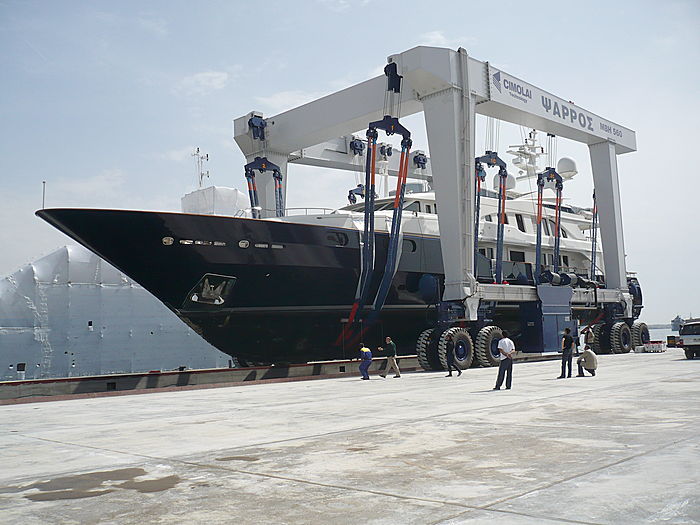
CASE STUDY
Cimolai Technology explains the business benefits it has achieved since the installation in terms of time savings in planning, and design, and improvements in product quality and in delivery forecast ability.
ansys mechanics rail-transport marine