Abstract
CFRP composites have been used in Automobili Lamborghini since 1983. Today, the main challenge is to reproduce their structural behavior by developing suitable numerical models whose set-up requires just simple experimental tests.
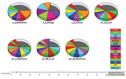
Automobili Lamborghini and EnginSoft started a collaboration to perfect sophisticated manufacturing applications and FE technical support with the aim to provide such numerical models. While the engineers relied on modeFRONTIER's capabilities, the procedure has been to calibrate the constitutive parameters of LS-DYNA's advanced material models, and to use them for prediction, design optimization and robustness analysis. In this way, the amount of expensive experimental tests could be reduced. This approach also allows better understanding of the influence of physical and geometrical variables on the composite dynamic structural response or, respectively, to obtain improved solutions for industrial case studies.
Read the article