Taking multi-stage steam turbine design beyond the barrier of perfection

Optimization Case study of a multi-stage steam turbine designed by Franco Tosi Meccanica

ABSTRACT

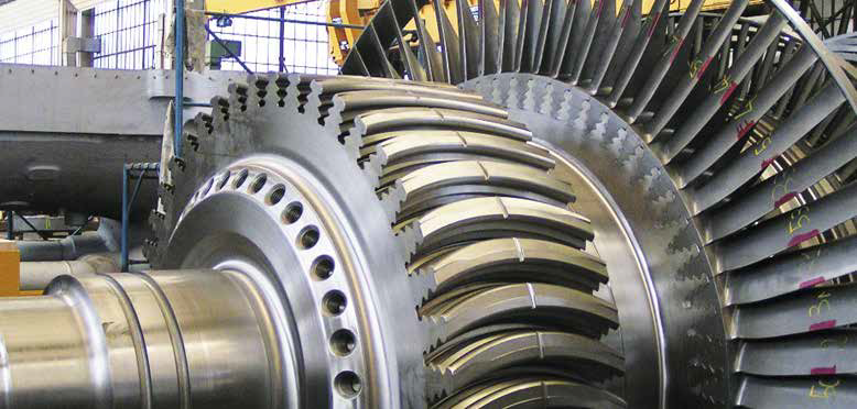
This case study details the design optimization of an axial steam turbine of 160 MW, focusing on maximizing the total-to-total isentropic efficiency of the last three low-pressure stages of the turbine. Specifically, the engineers considered the shape and angle of the blades. After more than one century of development, it is the advances in blade design that have contributed to improved steam turbine thermal efficiency. Since modern turbines already reach efficiency values beyond 90%, extracting any further improvement is a very challenging task. The engineers used a combination of three engineering approaches for this study to accomplish this: traditional trial-and-error, virtual optimization and direct optimization. The final verification of the steam turbine after the optimization, achieved an isentropic total-to-total efficiency gain of about 0.5% -- a small but vital improvement in today’s highly competitive, highly regulated market.